11. Testing Differential Expression across Multiple Samples

Even if expression appears high in one sample, you cannot tell whether it reflects individual variation, experimental noise, or the effect of a condition. You need multiple replicate samples to measure variation within each group before you can say that two groups are “statistically different.”

Question for this lesson: How do you test expression differences between two groups while accounting for variation across multiple samples?

The problem resembles trying to diagnose a latency regression from one measurement before deployment and one after. You must first know the ordinary variation among requests before deciding whether the deployment effect is larger. Differential expression replaces request repetitions with biological replicate samples and latency with raw counts for each gene.

Input table	Metadata	What the model separates	Output
gene × sample raw counts	Condition and batch for each sample	Group difference and within-group variation	log2FC, p-value, and padj for each gene

1. Moving to multiple samples: bulk RNA differential expression analysis

The fundamental limitation of one-sample (N=1) analysis is that it cannot estimate an ordinary range of variation. Individual and experimental differences can change expression, so a value that spikes in one sample cannot be separated statistically into a condition effect and ordinary variation.

Conventional bulk RNA analysis therefore uses multiple samples.

• It checks whether a specific change is reproduced across replicates.
• It compares samples with a normal control group and assigns statistical significance to each gene-level change.
• Experimental and control groups usually have at least n=3 each, the minimum needed to estimate variance, and more is better. Researchers sometimes collect the experimental group directly and use public data for the control group, in which case batch effects must be removed.

Workflow

Alignment and quantification follow the RNA-seq pipeline described earlier. Differential expression gene (DEG) analysis comes next.

FastQC → Trim Galore! → FastQC → STAR → featureCounts
      → DEG analysis (DESeq2 / limma-voom / edgeR)
      → visualization and functional analysis (Volcano plot, g:Profiler, GSEA)

• DEG analysis compares expression between two groups, such as Tumor vs Normal, one gene at a time. Its input is usually raw counts, before normalization.
• For each gene, it returns Log2FC, the fold change in expression between groups, and padj, a value adjusted for multiple testing. Reading DESeq2 and PyDESeq2 result tables explains the calculation relationships among columns from baseMean through padj, while Statistical testing and multiple testing explains the general difference between p-values and padj.
• The results can be plotted as a volcano plot, with Log2FC on the x-axis and significance on the y-axis, and the functions of standout gene sets can be interpreted with GSEA and g:Profiler.

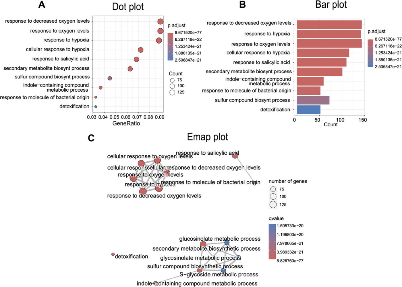
An example of enrichment visualizations, including a dot plot, bar plot, and enrichment map, that group genes selected by DEG analysis into functions or pathways. They summarize which biological programs differ between two groups.

What DESeq2 does

DESeq2, one of the most widely used DEG tools, performs the analysis in this order:

counts.shape       # genes × samples
sample_info.shape  # samples × conditions
results.shape      # genes × statistics

counts and sample_info must join exactly on sample ID. If column order is wrong and a condition label is attached to another sample, the model may run successfully while testing the wrong comparison. Validate IDs and ordering before analysis.

1. Connect the raw count matrix with condition information for each sample.
2. Remove genes with very low expression to reduce noise.
3. Correct for sequencing depth in each sample and estimate variation for each gene.
4. Test group differences with a model suited to count data, then calculate log2FC and padj.
5. Also produce variance-stabilized values for PCA and heatmaps.

🧩 Why raw counts? TPM converts values into within-sample proportions. DESeq2 takes raw counts because it needs to model variation in integer counts directly and correct for depth with its own method. What does DEG analysis test? explains the negative binomial distribution and the role of replicate samples in detail.

Moving from outlier detection with N=1 to statistical differential expression across multiple samples lets you go beyond “this gene spikes” and say that it changed in a statistically significant way.

Continue with the GSE251845 DEG exercise for a paired Tumour-Normal comparison within one cohort, or the EOCRC-LOCRC comparison exercise to estimate changes separately in two cohorts before comparing them.

Summary

Differential expression analysis is not about finding a large value in one sample. It accounts for within-group variation and sequencing depth to find genes that change consistently when the condition changes.

Replicate samples → raw counts → depth and variance estimation → group comparison → log2FC and significance → functional analysis